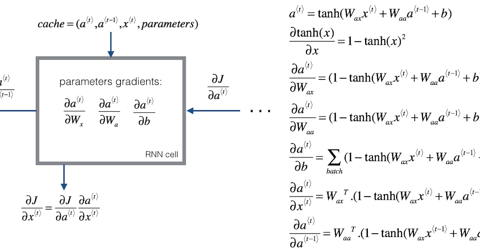
Recurrent Neural Networks

Introduction

Have you ever thought of how can I build an AI for a self-driving car so that it can predict the trajectory and avoid accidents or build an AI model which can predict a stock price and tell you when to buy or sell? Believe me, not this is quite similar to what we do on daily basis like catching a ball. I am sure you might be thinking how come to a simple task like catching a ball and predicting stock price be the same well in both of these problems, we are dealing with time series data. While catching the ball you look at the ball's previous trajectory and predict where the ball shall be in the next few seconds in the stocks model looks at the graphs do an analysis and look at the trajectory of the candle graph and conclude if to buy or sell.

In this series of blogs, I will be explaining RNN to you as well as myself. Generally, they are taking data of arbitrary length Ex. Music, text rather than fixed-sized data Ex. Images. This makes them extremely useful for NLP which is Natural Language Processing like text-to-speech analysis, sentiment recognition and language conversion.

I will be looking into the fundamental concept of RNN and the main issue of exploding and vanishing gradients and the solution namely:

1. LSTMS cells

2. GRU cells

Recurrent Neurons

So until now, I have read about feed-forward neural networks but RNN has backward connections too. Let's start with the simplest example as shown above. At a certain time-frame t the neuron as the inputs x(t) and y(t - 1) the input from the previous time frame. We can show this against the time axis its called 'unrolling the network through time'. Note that the output and the input here are vectors and not scalers like in a single NN. RNN has two weights w_x for input x(t) and w_y for y(t-1). The equation for output of a single neural network for a given instance can be given by it can be computed very easily as you might have expected (b is bais and ϕ(.) is activation function)

We can compute the output for the complete mini-batch by using a vectorized form of the above equation

NOTE: Remember the dimensions!

m --> number of instances in the mini-batch

n_neurons --> number of neurons

n_inputs --> number of input feature

Y(t) is m * n_neurons matrix containing the output of the layer at time step t for each instance of mini-batch

X(t) is m * n_input matrix containing the inputs for all instances

W_x is n_inputs * n_neurons containing the weight for the inputs of the current time step

W_y is n_neurons * n_neurons containing the weights for the outputs from the previous time step

W is the concatenation of weight matrices W_x and W_y and is of shape (n_input + n_neurons) * n_neurons

b is of shape n_neurons containing bais for each neuron

---

Prefer tanh() activation function in RNN rather than Relu()

---

If you look closely you will realize Y(t) is dependent on X(t) and Y(t - 1) and Y(t - 1) is dependent on X(t - 1) and Y(t - 2). Therefore, we can say that Y(t) is a function of X(t) where t = 0, 1, 2, ...... At t = 0 there is no previous output so we assume it to be 0

Memory Cell

The output of time step t is the function of previous time steps and their inputs we can say that it creates the memory of the previous states. The part of the neural net that preserves this state across time is called the Memory cell

The cell's hidden state is denoted as h(t) or a<t> and is a function of x(t) and h(t-1) ie. h(t) = f(x(t), h(t - 1)) and the output of this at t is given by y(t) which is also the function of the previous state and current inputs.

---

Updated equations:

Unlike above the y(t - 1) dose not determine y(t) but now h(t) does

W_h -> weights of the hidden state

W_hy -> weights of hidden state used to calculate y(t)

h(0) = 0

h(t) = g(W_h [h(t - 1) + X(t)] + b_h)

y(t) = g(W_yh * h(t) + b_y)

NOTE:

Shape of W_h is (No of Hidden neurons, No of Hidden neurons + n_x)

Shape of [h(t - 1) + X(t)] is (No of Hidden neurons + n_x, 1)

---

Until now we have been discussing the basic cells so the output is the same as the hidden state but it changes in complex cells

Back Propagation Through Time

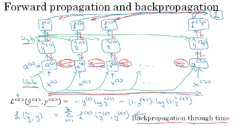
Usually, the programming framework takes care of backpropagation but it's always useful to understand it. We know that in forward propagation we have to compute these activations from left to right in NN and we have predictions for all outputs in backpropagation, we carry backpropagation calculation in the reverse direction of the propagation arrow. So in backpropagation, we just compute and parse messages in the reverse direction. As shown below compute y(t) and h(t) using W_y and W_h, after that we will compute loss for each time step ie L(t) and then let L = avg(L(1) ... L(t_y)) . Now in backpropagation, we will compute in direction of red arrows. The most significant calculation over here is the one in right to left direction. Here the time index decreases hence the name, backpropagation through time

Input and Output Sequence

The below-given diagram should make you understand the one-to-one network, sequence-vector(encoder) and vector-sequence(decoder) networks

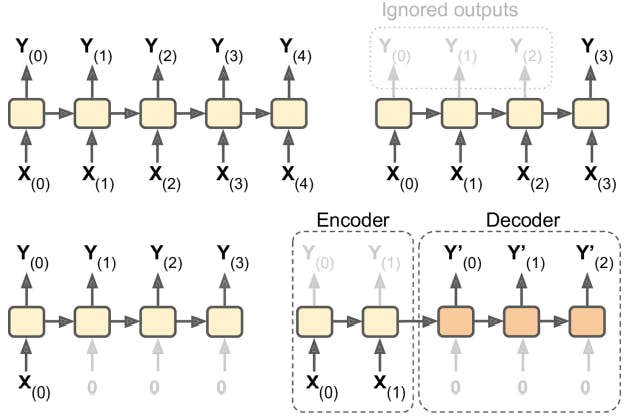
I am interested in the encoder-decoder network. For ex: We have to translate a sentence. So the encoder will convert the sentence (sequence) into a vector and this vector will be the input to the decoder which will output the translated sentence (sequence). In translation, even the last word may affect the first word so we cant use one-one network

Language model and Sequence Generation

Language modeling is a very important task of NLP and RNNs perform very well in it.

What is Language Modeling?

For example, we are building a speech recognition model and we say "The apple and pear salad" but what should be the output? "The apple and pair salad" or "The apple and pear salad". Here we take the help of the Language model. It tells us the probability of a particular sequence of words

Language Model with RNN

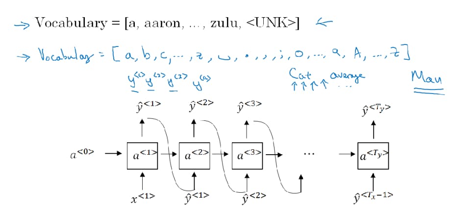
To train a model first we have to find training data set ie a large corpus of target language text, then tokenize it by getting the vocabulary and one hot encode each word. We can also use <EOS> for the end of a sentence and <UNK> for unknown words

RNN Model

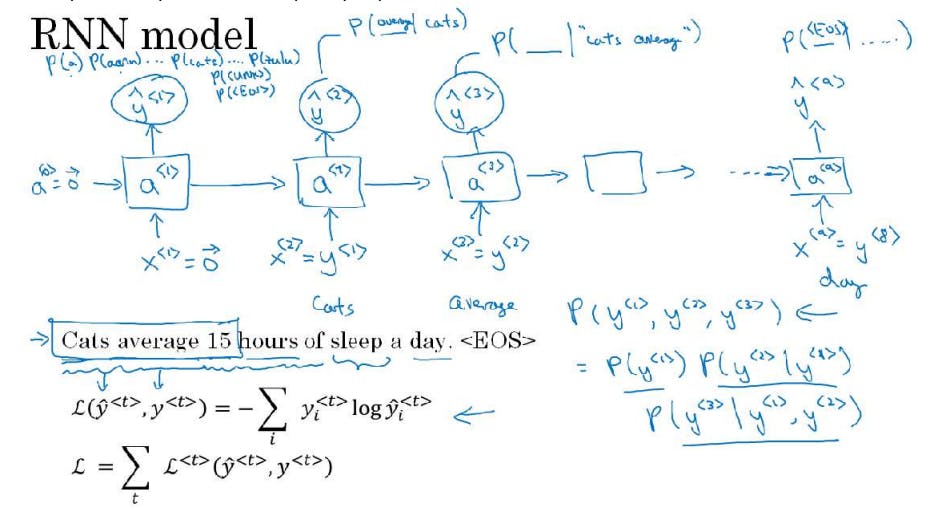
In the RNN model, we feed the sentence to it. but x(t) = y(t-1) ie the previous true output is the input to the neuron in the next time step. Here the model tries to predict the first word from the x(0)=0 and h(0) = 0 say it predicts it to be "dog" then we compute the loss and give the correct word ie. "cat" to the next time step neuron. It will then try to predict the next word given that the previous correct word was "cat".

To find the probability of a sentence y(1) y(2) y(3)

p(y, y, y ) = p(y ) * p(y | y ) * p(y | y, y ) . . . . . (Here we just feed the sentence to the model and multiply each word probability)

Sampling sequence from trained RNN

After the RNN model is trained, to understand informally what the model has learned we can apply it to sample novel sequences. Here let the model perform predictions as it used to but instead of giving it the true values we will give it randomly sampled values from our vocabulary using np. random. choice() which samples according to the distribution defined by the vector probabilities giving us a unique beginning for each sentence and passing the calculated h(1) to the next time step. Repeat this process until you reach <EOS> if the given prediction is <UNK> then ignore it and choose the next most probable output or remove it from your vocabulary if you don't want it.

Character Level Model

In the Character level model, the vocabulary consists of all the possible characters { a - z, A - Z, 0 - 9, punctuations, etc} instead of words. The character-level model doesn't need <UNK> token since vocabulary consists of all possible characters. But there are some disadvantages to it:

1. We end up with much longer sequences

2. Cant capture and use long-range dependencies effectively

3. Computationally expensive and is hard to train

Sequence Generation

The sentences your model generates highly depend on what kind of data you have used to train the model. The sentences generated by a model trained in news articles may seem quite formal whereas the sentences to the right are of a model trained in Shakespeare's literature and may seem quite poetic and archaic

In the next blog, we will be coding RNN with the help of tf

Sources:

1. Hands-On Machine Learning with Scikit-Learn & TensorFlow

2. Deep learning by Andrew Ng